Chapter 2 — Regression

From data to linear prediction models

Bryan G. Pantoja-Rosero

Chapter 2 — Regression

Learning relationships between numerical inputs and outputs

• What do we want to predict?
• What can the relationship tell us?
• How should we represent and fit a model?

1 THE REGRESSION PROBLEM

Regression relates input variables to a numerical output.

• Learn from known input–output examples.
• Predict output values for new inputs.
• Or study how outputs relate to inputs.

\[\hat y=f(\mathbf x)\approx y\]

Regression versus classification

• Regression: predict a numerical quantity.
  • Weight, sales, displacement, temperature.
• Classification: predict a category.
  • Damaged or undamaged building.
• Same broad learning framework; different output type.

Dataset for regression

\[ \mathcal D=\{(\mathbf x_n,y_n)\}_{n=1}^{N}, \]

• \((\mathbf x_n,y_n)\): one matched training pair.

One observation, \(D\) features

\[ \qquad \mathbf x_n=\begin{bmatrix}x_{n1}&x_{n2}&\cdots&x_{nD}\end{bmatrix}^{\!\top}\in\mathbb R^D, \qquad y_n\in\mathbb R. \]

• \(N\) observations (data-size); \(D\) features (dimensionality).
• \(n\): observation index.
• \(d\): feature index.

Dataset for regression

Dataset as a matrix

\[ X=\begin{bmatrix} x_{11}&\cdots&x_{1D}\\ \vdots&\ddots&\vdots\\ x_{N1}&\cdots&x_{ND} \end{bmatrix}\in\mathbb R^{N\times D},\qquad \mathbf y=\begin{bmatrix}y_1\\\vdots\\y_N\end{bmatrix}\in\mathbb R^N. \]

• Rows: observations.
• Columns: features.
• Each target \(y_n\) matches row \(n\) of \(X\).

A small tabular example

\(n\)	Height (cm)	Age (years)	Weight (kg)
1	160	22	58
2	173	28	71
3	185	24	82

• \(N=3\), \(D=2\).
• \(\mathbf x_2=(173,28)^\top\); \(y_2=71\).
• Remove age → \(D=1\); \(N\) is unchanged.

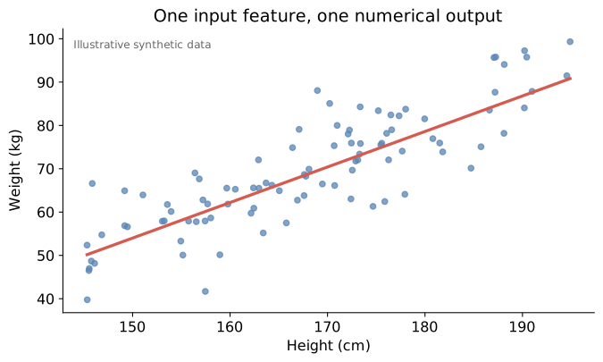
Example: height and weight

Schematic height–weight regression. Synthetic observations.

• Univariate regression: one input feature.
• Association visible; points do not all lie on one line.

Do we know the right shape?

• The dataset is observed before the model is chosen.
• A trend may look linear, nonlinear, or noisy.
• A straight line is a modeling assumption, not a property guaranteed by the data.

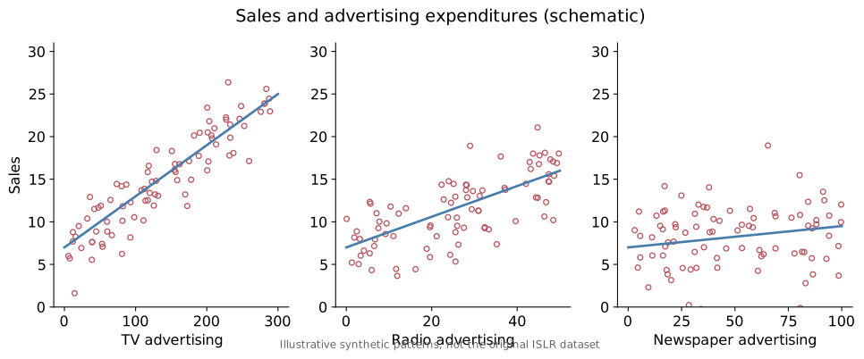
Example: advertising and sales

Illustrative relationships between sales and advertising expenditures.

• Inputs: TV, radio, newspaper spending.
• Output: sales.
• Three features can be used jointly in one model.

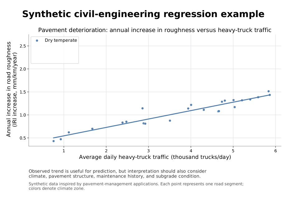
Engineering example: pavement deterioration

Heavy-truck traffic and pavement deterioration grouped by climatic conditions. Synthetic observations.

• Input: daily heavy-truck traffic.
• Target: annual increase in pavement roughness.
• Higher traffic often accompanies faster deterioration.

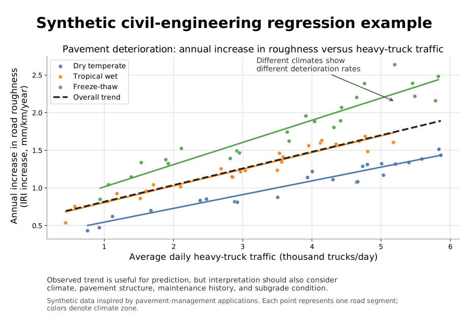
Why do pavement trends differ?

Heavy-truck traffic and pavement deterioration grouped by climatic conditions. Synthetic observations.

• Climate, drainage, pavement structure, construction quality and maintenance history.
• Same truck traffic ≠ same deterioration rate.
• Prediction can help plan maintenance; interpret with care.

Two goals of regression

Prediction

• What is the weight of someone 170 cm tall?
• What displacement is expected under a given load?
• Priority: accuracy on new inputs.

Interpretation

• Are taller people generally heavier?
• How does predicted response vary with load?
• Priority: understanding relationships.

A model function

For both goals, introduce a regression function \(f\) and seek predictions:

\[ \hat y_n=f(\mathbf x_n)\approx y_n, \qquad n=1,\ldots,N. \]

When function is controlled by numerical parameters \(\mathbf w\):

\[ \boxed{\hat y_n=f_{\mathbf w}(\mathbf x_n)} \qquad or \qquad \boxed{\hat y_n=f_{\mathbf w}(\mathbf x_n, \mathbf w)} \]

• \(\mathbf x_n\): input features.
• \(y_n\): observed target.
• \(\hat y_n\): model prediction.
• \(\mathbf w\): adjustable parameters.

Two choices: choose the form of \(f\); then fit \(\mathbf w\).

2 LINEAR REGRESSION

Linear regression represents the predicted output as a linear combination of input features, usually with an additional constant term.

Why linear regression?

• Simple mathematical form.
• Parameters are relatively easy to interpret.
• Efficient numerical predictions.
• Introduces concepts shared with more advanced models.

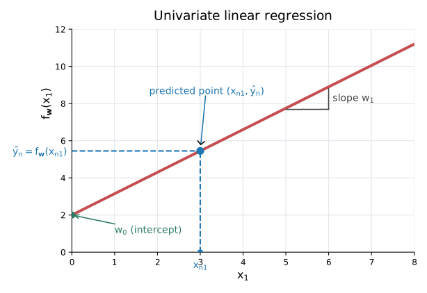
Univariate linear regression

\[ \boxed{\hat y_n=f_{\mathbf w}(x_n)=w_0+w_1x_{n1}.} \]

• \(w_0\): intercept / offset.
• \(w_1\): slope.
• Two parameters, one input feature.

Univariate linear regression

Geometry: slope and intercept

Slope and intercept in linear regression.

• \(w_0=f(0)\).
• \(w_1=\Delta\hat y/\Delta x\).
• Slope units: output units / input units.

Univariate linear regression

Toy example: load and displacement

\[\hat y=1+0.4x\]

• \(x\): load (kN); \(\hat y\): displacement (mm).
• \(x=10\) kN → \(\hat y=5\) mm.
• Slope: 0.4 mm/kN.
• Is the intercept physically meaningful?

Illustrative equation; not a calibrated structural model.

Multivariate linear regression

\[ \begin{aligned} \hat y_n=f_{\mathbf w}(\mathbf x_n) &=w_0+w_1x_{n1}+w_2x_{n2}+\cdots+w_Dx_{nD} \end{aligned} \] \[ \boxed{\hat y_n=w_0+\sum_{d=1}^{D}w_dx_{nd}=w_0 + {\mathbf x}_n^\top{\mathbf w}} \]

• \(D\) observed input features; but \(D+1\) parameters with intercept.
• \(w_d\): coefficient on feature \(d\).

Multivariate linear regression

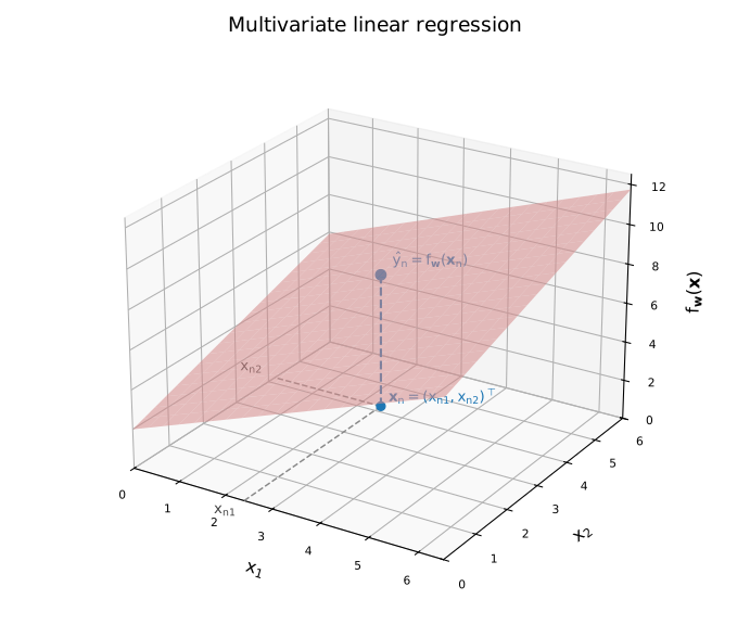
Two features: a prediction plane

A plane models a numerical output from two input features.

\[\hat y_n=w_0+w_1x_{n1}+w_2x_{n2}\]

Multivariate linear regression

Reading multivariate coefficients (load+temperature vs displacement)

• Example inputs: load \(x_1\), temperature \(x_2\).

\[\hat y_n=1+0.4x_{n1}+0.01x_{n2}\]

• Prediction changes by \(w_1\Delta x_1\) when \(x_2\) is held fixed.
• A model coefficient describes a modeled association.
• Not automatically a causal effect.

Augmented feature vector

\[ \boxed{\hat y_n=w_0+\sum_{d=1}^{D}w_dx_{nd}=w_0 + {\mathbf x}_n^\top{\mathbf w}} \]

Why add a feature equal to 1?

\[ \tilde{\mathbf x}_n=\begin{bmatrix}1\\x_{n1}\\\vdots\\x_{nD}\end{bmatrix},\qquad \tilde{\mathbf w}=\begin{bmatrix}w_0\\w_1\\\vdots\\w_D\end{bmatrix} \]

• The leading 1 is a synthetic constant feature.
• It incorporates the intercept into one operation.
• Both vectors have \(D+1\) entries.

Augmented feature vector

One dot product — whole prediction

\[ \boxed{\hat y_n=\tilde{\mathbf x}_n^\top\tilde{\mathbf w}} \]

\[=1\cdot w_0+x_{n1}w_1+\cdots+x_{nD}w_D\]

• Same model, more compact notation.
• Dot products are efficient computational building blocks.

Check the dot product

\[\tilde{\mathbf x}=\begin{bmatrix}1\\2\\3\end{bmatrix},\qquad \tilde{\mathbf w}=\begin{bmatrix}4\\1.5\\-2\end{bmatrix}\]

\[\hat y=4+2(1.5)+3(-2)=\boxed{1}\]

Question: How would you write the equation without augmented vectors?

Augmented feature vector

All observations in one operation

\[ \tilde X=\begin{bmatrix} 1&x_{11}&\cdots&x_{1D}\\ 1&x_{21}&\cdots&x_{2D}\\ \vdots&\vdots&\ddots&\vdots\\ 1&x_{N1}&\cdots&x_{ND} \end{bmatrix}\in\mathbb R^{N\times(D+1)}. \]

\[\boxed{\hat{\mathbf y}=\tilde X\tilde{\mathbf w}\in\mathbb R^N}\]

• Each row yields one predicted output.
• Inner dimensions \(D+1\) must match.
• Enables efficient batch predictions.

Learning and fitting the model

Definition: write the function \(f_{\mathbf w}\) \(\neq\) find the best model for the observations.

Fitting (or estimation or learning): find optimal parameter values \(\mathbf w\) given data \((x_n, y_n)\).

• Different parameters → different lines or planes.
• Need a criterion for comparing their predictions.
• Next: loss functions and optimization.

Learning and fitting the model

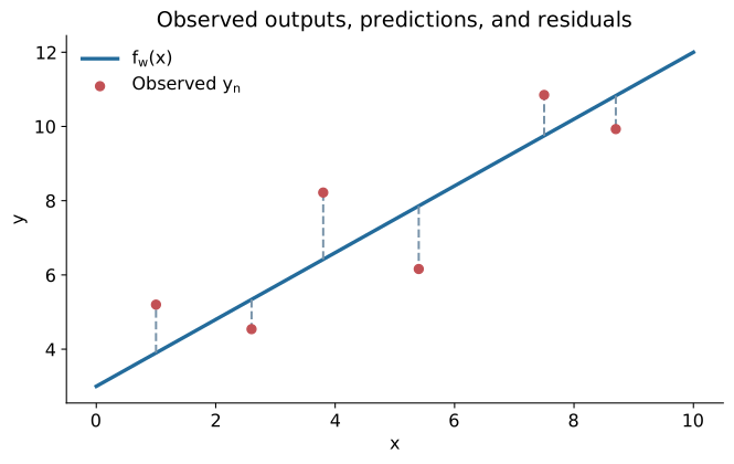
Predictions and residuals

\[\boxed{e_n=y_n-\hat y_n}\]

Observed values, predicted values, and residuals.

• Positive residual: underprediction.
• Negative residual: overprediction.

Learning and fitting the model

How can parameters be learned?

• Compare predictions \(\hat y_n\) with observed \(y_n\).
• Combine discrepancies through a loss function.
• Adjust parameters using an optimization method.
• Gradient-based methods use how loss changes with parameters.

Later chapters: formal loss definitions and optimization algorithms.

Error magnitude: a preview of MSE

\[ \mathrm{MSE}=\frac{1}{N}\sum_{n=1}^{N}(y_n-\hat y_n)^2 =\frac{1}{N}\sum_{n=1}^{N}e_n^2. \]

Overparameterization and non-unique solutions

A fundamental question: enough data?

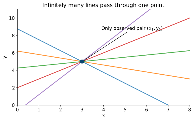
• What happens with one observation and a two-parameter line?
• Can we draw a line through the point? Is that line unique? \[y_1=w_0+w_1x_1\]

Overparameterization and non-unique solutions

Infinitely many perfect fits

Different lines through the same one training point.

\[\boxed{w_0=y_1-w_1x_1}\]

• Choose any slope → adjust intercept.
• Training data do not identify a unique model.

Overparameterization and non-unique solutions

Overparameterization: \(D>N\)

• With intercept, linear regression has \(D+1\) parameters.
• If \(N<D+1\): insufficient independent equations for unique parameters.
• Often called underdetermined or overparameterized.
• Even \(N\ge D+1\) can be insufficient if features are dependent.

Overparameterization and non-unique solutions

More parameters: always bad?

• \(N<D+1\): parameters cannot be uniquely identified.
• Even \(N\ge D+1\): dependent features may prevent uniqueness.
• Extra model flexibility does not guarantee a better physical model.
• Large modern models can nevertheless generalize.
• Training fit ≠ performance on unseen cases.
• Later: overfitting, regularization, evaluation.

Example: Concrete compressive strength (2D)

• Input: cement content (kg/m³). Target: 28-day concrete compressive strength (MPa).

Example: Concrete compressive strength (3D)

• Inputs: cement and water content (kg/m³). Target: 28-day concrete compressive strength (MPa).

Example: Concrete compressive strength

What did the interactives show?

• 1 feature: a line in the \((x,y)\) plane.
• 2 features: a plane in \((x_1,x_2,y)\) space.
• Changing coefficients changes predictions and residuals.
• A better training fit does not automatically mean better generalization.
• Next question: how can parameter fitting be automated?

Correlation is not causation

Statistical association ≠ causal effect.

• Shared drivers: a third variable influences both quantities.
• Shared trends: unrelated variables change over time.
• Coincidence: apparent patterns in finite datasets.
• In scientific and engineering applications, predicting an outcome is different from explaining what causes it.
• Causation requires additional evidence and an understanding of the physical mechanisms involved.
• Results must be interpreted alongside domain knowledge.

Confounding: an engineering example

• Observed: electricity use ↑; maintenance costs ↑.
• Does electricity consumption cause higher maintenance cost?
• Larger buildings may have both higher consumption and higher costs.
• Building size: possible confounding variable.

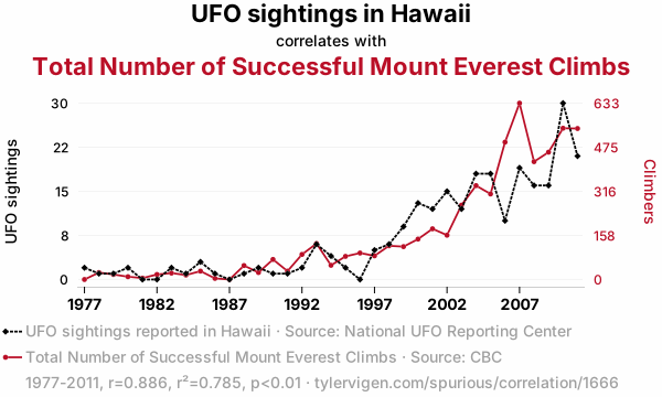
Spurious correlations — example 1

UFO sightings in Hawaii and successful Mount Everest climbs, 1977–2011. Source: Tyler Vigen, Spurious Correlations (https://www.tylervigen.com/spurious/correlation/1666).

• Strong common trend; no credible causal connection.

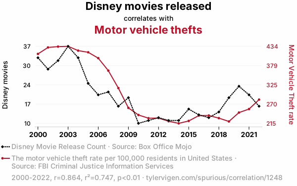
Spurious correlations — example 2

Disney movie releases and US motor vehicle thefts, 2000–2022. Source: Tyler Vigen, Spurious Correlations (https://www.tylervigen.com/spurious/correlation/1248).

• Similar historical variation does not imply causation.

Regression terminology

Input side	Output side
Feature	Target
Predictor	Response
Covariate	Outcome
Independent variable	Dependent variable
Regressor	Regressand

Some disciplinary terms carry additional technical assumptions.

A model without an offset

\[\hat y_n=\mathbf x_n^\top\mathbf w\]

• \(D\) parameters, rather than \(D+1\).
• Forces \(\hat y=0\) when all inputs are zero.
• Choose only if that restriction is appropriate.
• In neural networks, parameter count can differ greatly from \(D\).

Matrix multiplication refresher

\[\boxed{A_{M\times N}\,B_{N\times D}=C_{M\times D}}\]

• Inner dimensions must match.
• Output shape: outer dimensions.

\[C_{ij}=\sum_{k=1}^{N}A_{ik}B_{kj}\]

Coming next

Loss functions

• How should we quantify prediction errors?
• What makes one set of parameters better than another?

Then: optimization

• How can we systematically learn parameters?

Acknowledgements and AI Disclosure

Acknowledgements

• Developed with reference to CS-433 Machine Learning, École Polytechnique Fédérale de Lausanne (EPFL).
• Adapted and extended for the present course, including civil engineering applications.
• Independent teaching materials; no EPFL endorsement is implied.
• Original EPFL course

Use of Generative AI

• AI-assisted drafting, editing, examples, figures, and interactive visualizations.
• The instructor is responsible for the final content and technical accuracy.
• External materials are acknowledged separately.