Chapter 3 — Loss Functions
Measuring prediction errors and choosing learning objectives
1 Chapter overview
In Chapter 2, a regression model transformed an input vector \(\mathbf x_n\) into a numerical prediction \(\hat y_n=f_{\mathbf w}(\mathbf x_n)\). Different parameter values produce different predictions, but the equation alone does not tell us which parameters fit the observed data best. How can we quantify the quality of a model and compare different choices of parameters?
A loss function converts the discrepancy between a prediction and its target into a numerical cost. Combining the losses across observations yields an objective that can be minimized during learning. This chapter develops that idea, examines mean squared error (MSE) and mean absolute error (MAE) using the same numerical example, and investigates their sensitivity to outliers. Finally, it introduces convexity as a property that helps us understand whether minimizing a loss is computationally manageable. The central lesson is that choosing a loss involves both statistical considerations and computational considerations.
1.1 Learning objectives
By the end of this chapter, you should be able to:
- Distinguish an observed target, a prediction, a signed residual, an individual loss, and a dataset-level objective.
- Define and interpret MSE and MAE for regression.
- Compute both losses for a constant prediction model and compare candidate parameters.
- Explain how an outlier can affect a fitted model differently under MSE and MAE.
- Discuss desirable loss properties, including symmetry, robustness, and ease of optimization.
- Explain convexity geometrically and mathematically, and describe why convex objectives are valuable.
- Recognize the role of the model and loss function in determining convexity with respect to parameters.
- Explain why the choice of loss must reflect the practical consequences of prediction errors.
2 Why do we need a loss function?
Consider two regression models for a numerical target. A simple one-parameter model predicts the same constant for every observation, regardless of the input:
\[ \hat y_n=f_{w_0}(\mathbf x_n)=w_0. \]
A two-parameter model with one input feature can adjust its prediction according to the value of that feature:
\[ \hat y_n=f_{\mathbf w}(x_{n1})=w_0+w_1x_{n1}, \qquad \mathbf w=(w_0,w_1)^\top. \]
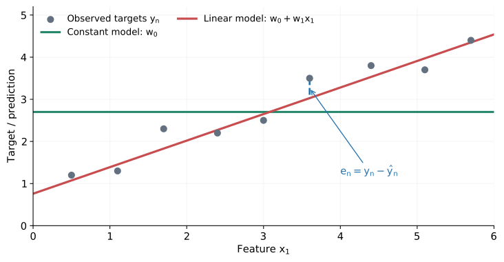
The constant model produces a horizontal line; the second model produces a line whose slope and intercept can vary. Either may fit a particular dataset better, depending on the observations and parameter values. Comparing them requires a criterion beyond a visual impression of the plotted lines.
2.1 From residuals to losses
For observation \(n\), let \(\mathbf x_n\) denote the input and \(y_n\) the measured or observed target. Given model parameters \(\mathbf w\), the prediction is \(\hat y_n=f_{\mathbf w}(\mathbf x_n)\). As introduced in Chapter 2, the residual is
\[ \boxed{e_n=y_n-\hat y_n=y_n-f_{\mathbf w}(\mathbf x_n).} \]
A positive residual indicates that the prediction was too low; a negative residual indicates that it was too high. The residual retains the direction of the error, but its sign makes it unsuitable as a cost by itself: positive and negative residuals could cancel when summed. We therefore introduce a function \(\ell\) that assigns a numerical individual loss to an error:
\[ \ell(e_n)=\ell\!\left(y_n-f_{\mathbf w}(\mathbf x_n)\right). \]
The loss specifies how costly a particular mistake is. For example, it may assign the same cost to residuals \(+3\) and \(-3\), or treat one direction of error as more serious. This choice depends on what we want the model to accomplish.
To evaluate the model on the full dataset \(\mathcal D=\{(\mathbf x_n,y_n)\}_{n=1}^{N}\), we combine the individual losses. A common choice is their average:
\[ \boxed{L(\mathbf w)=\frac{1}{N}\sum_{n=1}^{N}\ell\!\left(y_n-f_{\mathbf w}(\mathbf x_n)\right) =\frac{1}{N}\sum_{n=1}^{N}\ell(e_n).} \]
This is the dataset loss, also called the cost function, training objective, or simply the objective function. It is a single number determined by the observations, model, parameters, and chosen individual loss. For a fixed training dataset, it is useful to view \(L\) as a function of the adjustable parameters \(\mathbf w\). Learning consists of searching for parameters that make this objective sufficiently small:
\[ \mathbf w^*\in\operatorname*{arg\,min}_{\mathbf w}L(\mathbf w). \]
The notation \(\operatorname*{arg\,min}\) denotes the set of parameter values attaining the smallest loss, when a minimum exists. There can be more than one such value. Defining the loss and minimizing it are distinct tasks: first we decide what counts as a good prediction, and then we determine how to achieve it.
3 Desirable properties of loss functions
Not all losses treat mistakes in the same way. In regression with real-valued targets, several characteristics are useful to consider.
Nonnegative costs and a minimum at zero. It is natural for a perfect prediction, \(e=0\), to have zero loss and for errors to incur a nonnegative cost. This convention makes smaller values easier to interpret as better fits, although every possible application need not follow exactly the same convention.
Symmetry around zero. A symmetric loss obeys \(\ell(e)=\ell(-e)\), so underpredicting by a given amount costs the same as overpredicting by that amount. Both squared and absolute error have this property. Symmetry is often appropriate for a basic regression problem, but it is not compulsory: in some applications, an underprediction may be more costly than an equally large overprediction.
Sensitivity to large errors. A loss should indicate when a prediction is far from its target, but the rate at which the penalty increases matters. If one unusually large residual overwhelms the losses from all other observations, it may pull the fitted model away from the pattern represented by the majority of the data. This motivates statistical robustness: limiting the effect of a small number of atypical observations on the learned model.
Computational convenience. We must also be able to find parameter values with low loss. Smoothness, differentiability, and—especially for the models considered here—convexity influence how easy it is to optimize the dataset objective. A statistically attractive loss may be difficult to minimize, whereas an easy-to-optimize loss may react poorly to outliers. This is an important practical trade-off rather than a rule that every robust loss must be non-convex.
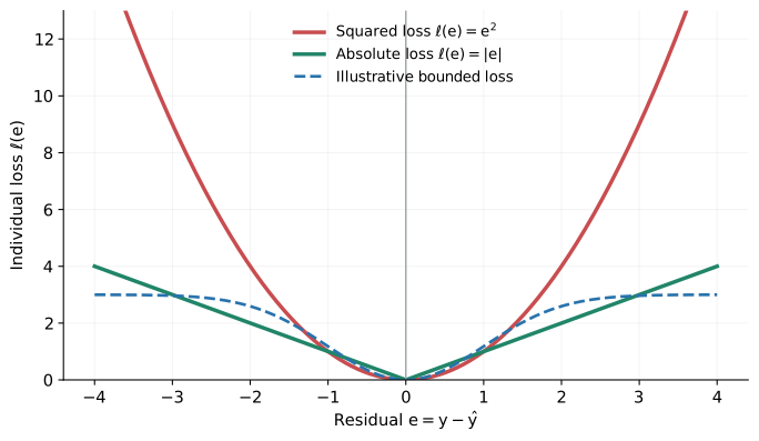
The two principal losses developed below illustrate these differences directly. Squared error penalizes large mistakes increasingly strongly, whereas absolute error increases linearly with their magnitude.
4 Mean squared error (MSE)
For an individual observation, the squared loss is
\[ \boxed{\ell_{\mathrm{SE}}(e_n)=e_n^2=(y_n-\hat y_n)^2.} \]
Averaging this quantity over all observations gives the mean squared error:
\[ \boxed{\mathrm{MSE}(\mathbf w)=\frac{1}{N}\sum_{n=1}^{N}\left(y_n-f_{\mathbf w}(\mathbf x_n)\right)^2 =\frac{1}{N}\sum_{n=1}^{N}e_n^2.} \]
Squaring eliminates the sign, makes MSE nonnegative, and assigns the same cost to positive and negative residuals of equal magnitude. Importantly, the cost increases quadratically with the residual: an error twice as large contributes four times as much squared loss. This property makes MSE widely used and mathematically convenient, but it also increases the influence of very large errors.
4.1 Worked example: fitting a constant model
Consider the one-parameter model \(\hat y_n=w_0\), which predicts the same value for every observation. Suppose the observed targets are
\[ (y_1,y_2,y_3,y_4)=(1,2,3,4),\qquad N=4. \]
Because the prediction does not depend on the input, the individual squared loss is \((y_n-w_0)^2\). The dataset objective is
\[ \mathrm{MSE}(w_0)=\frac14\left[(1-w_0)^2+(2-w_0)^2+(3-w_0)^2+(4-w_0)^2\right]. \]
We can compare candidate values of \(w_0\) without yet using an optimization algorithm. For example, choosing \(w_0=1\) gives squared errors \(0,1,4,9\); their sum is \(14\) and their mean is \(14/4=3.5\). Choosing \(w_0=2\) gives squared errors \(1,0,1,4\), summing to \(6\) and averaging to \(1.5\).
| Candidate \(w_0\) | 1 | 2 | 3 | 4 | 5 | 6 | 7 |
|---|---|---|---|---|---|---|---|
| \(\sum_{n=1}^{4}(y_n-w_0)^2\) | 14 | 6 | 6 | 14 | 30 | 54 | 86 |
| \(\mathrm{MSE}(w_0)\) | 3.5 | 1.5 | 1.5 | 3.5 | 7.5 | 13.5 | 21.5 |
Among the integer candidate values shown, \(w_0=2\) and \(w_0=3\) tie for the smallest MSE. If any real-valued parameter is allowed, the true minimum occurs at \(w_0=2.5\), the mean of the four targets. This distinction matters: a finite table compares only the candidates included in the table; it does not necessarily locate the optimum over all real numbers.
4.2 What happens when an outlier is added?
Now suppose we add a fifth observation with the unusually high target \(y_5=20\). The original four targets remain unchanged, but the objective becomes
\[ \mathrm{MSE}_{\mathrm{new}}(w_0)=\frac15\left[\sum_{n=1}^{4}(y_n-w_0)^2+(20-w_0)^2\right]. \]
The new observation contributes a large squared error when \(w_0\) remains near the original values. For example, at \(w_0=2\), its contribution alone is \((20-2)^2=324\). The sums below make the effect visible.
| Candidate \(w_0\) | 1 | 2 | 3 | 4 | 5 | 6 | 7 |
|---|---|---|---|---|---|---|---|
| Original squared-error sum | 14 | 6 | 6 | 14 | 30 | 54 | 86 |
| Outlier contribution \((20-w_0)^2\) | 361 | 324 | 289 | 256 | 225 | 196 | 169 |
| New squared-error sum | 375 | 330 | 295 | 270 | 255 | 250 | 255 |
Among these candidates, the lowest total is now obtained at \(w_0=6\). In fact, the minimum over all real-valued values is also \(w_0=6\), the new target mean \((1+2+3+4+20)/5\). One additional extreme observation moved the optimal constant prediction from \(2.5\) to \(6\).

The change illustrates why MSE is sensitive to outliers. A very large residual has a disproportionate effect because it is squared. An extreme observation may be a genuine but unusual case, a faulty measurement, or a data-processing error; the loss function alone cannot decide which interpretation is correct.
5 Outliers and measurement data
An outlier is an observation that lies unusually far from the bulk of the data. There is no universally applicable threshold: deciding whether a value is anomalous depends on the distribution of the data and knowledge of the measurement process. Unusual observations can arise from faulty sensors, recording mistakes, labeling errors, or genuinely uncommon events.
A historical example concerns Simon Newcomb’s measurements associated with the speed of light, later used in discussions of robust statistical methods. Most recorded deviations were concentrated within a relatively narrow range, while a few values, notably \(-44\) and \(-2\) in the dataset’s recorded units, lay well below the main cluster. These are deviations in the historical measurement notation, not negative physical speeds of light.
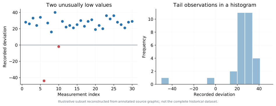
Their presence motivates an important modeling question: Should a handful of unusual measurements be allowed to dominate the fitted model? There is no answer independent of the application. Sometimes the rare events are precisely what we care about; in other cases they reflect unreliable data. A useful loss function must balance sensitivity to meaningful errors with resistance to unwanted distortion from atypical observations.
6 Mean absolute error (MAE)
A second widely used choice is the absolute loss:
\[ \boxed{\ell_{\mathrm{AE}}(e_n)=|e_n|=|y_n-\hat y_n|.} \]
Averaging over the dataset gives the mean absolute error:
\[ \boxed{\mathrm{MAE}(\mathbf w)=\frac1N\sum_{n=1}^{N}\left|y_n-f_{\mathbf w}(\mathbf x_n)\right| =\frac1N\sum_{n=1}^{N}|e_n|.} \]
Like MSE, MAE is nonnegative and symmetric around zero. Unlike MSE, it increases linearly with the size of the error. Doubling the magnitude of an error doubles its contribution to the total absolute loss, instead of quadrupling it. As a result, MAE is less sensitive to very large residuals than MSE in many fitting problems.
6.1 Repeating the constant-model exercise
Using exactly the same four targets, \((1,2,3,4)\), and the same constant model \(\hat y_n=w_0\), we now minimize
\[ \mathrm{MAE}(w_0)=\frac14\left[|1-w_0|+|2-w_0|+|3-w_0|+|4-w_0|\right]. \]
For the candidate values previously examined, the sum of absolute errors is:
| Candidate \(w_0\) | 1 | 2 | 3 | 4 | 5 | 6 | 7 |
|---|---|---|---|---|---|---|---|
| \(\sum_{n=1}^{4}|y_n-w_0|\) | 6 | 4 | 4 | 6 | 10 | 14 | 18 |
| \(\mathrm{MAE}(w_0)\) | 1.5 | 1 | 1 | 1.5 | 2.5 | 3.5 | 4.5 |
Again, \(w_0=2\) and \(w_0=3\) are best among these integer candidates. In fact, for the four observations, every value in the interval \([2,3]\) minimizes MAE. This interval is the set of medians of the four targets.
With the fifth target \(20\), we instead obtain:
| Candidate \(w_0\) | 1 | 2 | 3 | 4 | 5 | 6 | 7 |
|---|---|---|---|---|---|---|---|
| Original absolute-error sum | 6 | 4 | 4 | 6 | 10 | 14 | 18 |
| Outlier contribution \(|20-w_0|\) | 19 | 18 | 17 | 16 | 15 | 14 | 13 |
| New absolute-error sum | 25 | 22 | 21 | 22 | 25 | 28 | 31 |
The new optimum is \(w_0=3\), the median of the five values \((1,2,3,4,20)\). In contrast to MSE, adding the outlier moves the MAE optimum only from the interval \([2,3]\) to its endpoint \(3\).
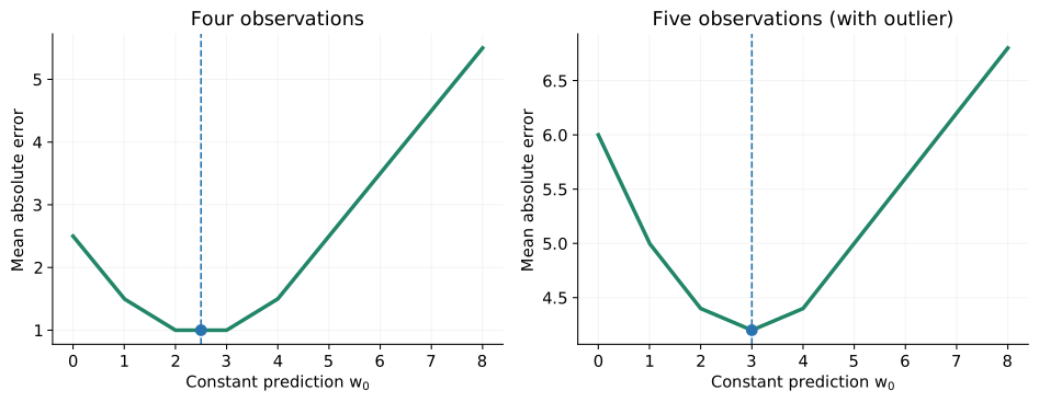
This comparison exposes a characteristic difference between the two losses for a constant model: squared error is minimized by the mean, whereas absolute error is minimized by a median. Because the mean can shift substantially when an extreme observation is added, MSE may produce a large change in the fitted constant. The median is generally less affected by the magnitude of a single extreme value. This does not mean MAE is always the correct choice, only that it offers a different treatment of the same data.
6.2 Comparing MSE and MAE
| Property | Mean squared error | Mean absolute error |
|---|---|---|
| Individual penalty | \(e^2\) | \(|e|\) |
| Growth with \(|e|\) | Quadratic | Linear |
| Equal cost for \(+e\) and \(-e\)? | Yes | Yes |
| Constant-model minimizer | Mean target | Median target (possibly non-unique) |
| Influence of large residuals | Stronger | More controlled |
| Shape near \(e=0\) | Smooth | Corner; not differentiable at zero |
| Convex as a function of \(e\) | Yes | Yes |
The computational distinction is also relevant. Squared loss has an ordinary derivative everywhere, whereas absolute loss has a corner at zero. This makes the squared loss especially convenient for gradient-based optimization, although MAE can also be optimized using appropriate methods. In fact, for a linear prediction model, both MSE and MAE lead to convex objectives. Robustness and computational convenience are therefore related considerations, but not a strict either–or choice.
7 Choosing a loss for the actual problem
A mathematical loss is not only a formula; it encodes what constitutes a costly mistake. For a basic numerical prediction problem, we might penalize overpredictions and underpredictions equally. In a decision-making problem, however, the consequences can be asymmetric. Incorrectly approving a financial loan and incorrectly rejecting one may have different costs, for example. More generally, the objective should reflect the specific practical decision being supported.
Engineering applications make this distinction equally clear. Predicting a structural response too low and predicting it too high may have different consequences if the predictions are subsequently used for safety-related decisions. Such an asymmetry cannot be captured solely by assuming the same penalty for \(e\) and \(-e\). It requires explicitly deciding which prediction errors matter and how they should be valued. This is a motivation for the choice of loss, not a new loss function derived in this chapter.
Losses also allow us to evaluate a fitted model on separate datasets. Computing the same quantity on the observations used for fitting produces a training loss; computing it on held-out observations gives a validation loss. These values help distinguish fitting the available examples from producing predictions on new cases, although careful generalization assessment involves additional considerations developed later. Similar principles extend beyond regression to classification and other prediction tasks: to train and evaluate a model, we must define how its outputs will be judged.
8 Convexity: a useful computational property
A loss must not only represent what we care about; its associated objective should ideally be manageable to minimize. This motivates the concept of convexity.
8.1 Geometric and mathematical definition
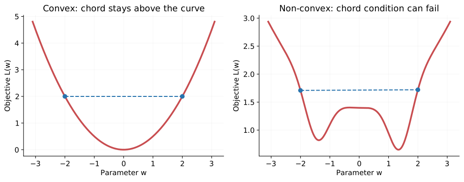
A function \(h:\mathbb R^D\to\mathbb R\) is convex when the straight line segment joining any two points on its graph lies on or above the graph. In mathematical terms, for any \(\mathbf u,\mathbf v\in\mathbb R^D\) and any \(\lambda\in[0,1]\),
\[ \boxed{h\!\left(\lambda\mathbf u+(1-\lambda)\mathbf v\right) \leq \lambda h(\mathbf u)+(1-\lambda)h(\mathbf v).} \]
The expression inside \(h\) on the left is an intermediate point between \(\mathbf u\) and \(\mathbf v\). The right-hand side is the corresponding linear interpolation between their function values. If the function never rises above that interpolating line, it is convex.
A function is strictly convex when this inequality is strict for distinct \(\mathbf u\ne\mathbf v\) and \(0<\lambda<1\). Both \(e^2\) and \(|e|\) are convex in the scalar residual \(e\), although \(|e|\) is not strictly convex over the whole real line.
8.2 Why convexity is valuable
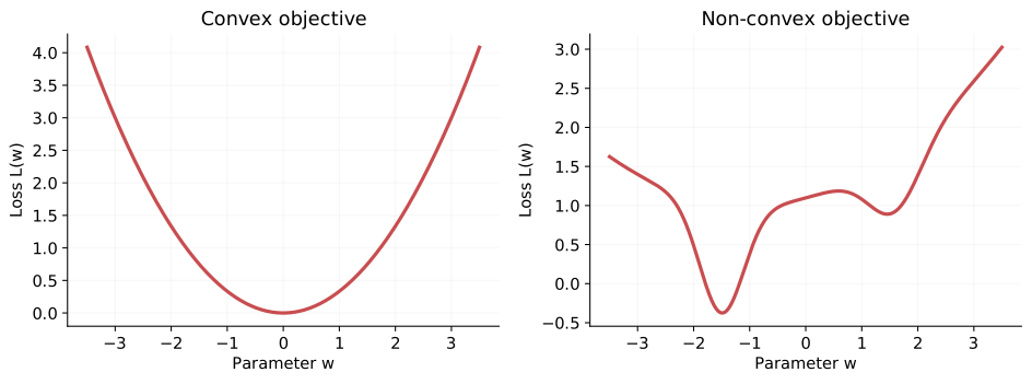
For a convex objective \(L(\mathbf w)\), every local minimum is also a global minimum. In particular, if optimization reaches a local minimum, there is no better minimum elsewhere in the parameter domain. By contrast, a non-convex objective can have several local minima with different loss values. An algorithm that moves toward lower loss may stop at one of these without reaching the lowest possible value.
Strict convexity gives a stronger guarantee: if a strictly convex function attains a minimum, that minimizer is unique. A merely convex function may have multiple minimizers, as in the flat minimum of MAE for the four-target example. Convexity does not by itself guarantee that a minimum exists; the existence of a minimizer also matters.
8.3 Convexity must be assessed in the model parameters
There is an important distinction between a loss \(\ell(e)\) as a function of the residual and the full objective \(L(\mathbf w)\) as a function of model parameters. When we fit the model, we optimize the parameters; therefore, it is convexity with respect to \(\mathbf w\) that matters.
For example, consider a linear model without an intercept,
\[ \hat y_n=f_{\mathbf w}(\mathbf x_n)=\mathbf x_n^\top\mathbf w. \]
The squared-error objective is then
\[ L_{\mathrm{MSE}}(\mathbf w)=\frac1N\sum_{n=1}^{N}\left(y_n-\mathbf x_n^\top\mathbf w\right)^2. \]
Each residual \(y_n-\mathbf x_n^\top\mathbf w\) is an affine function of \(\mathbf w\). Squaring it produces a convex function of \(\mathbf w\), and a sum of convex functions is convex. Consequently, MSE combined with a linear model is convex in its parameters. The same reasoning applies when an intercept is included through the augmented feature vector \(\tilde{\mathbf x}_n\).
Importantly, convexity does not imply a unique MSE solution in every dataset. If there are redundant features or insufficient independent observations, the squared-loss objective can be convex without being strictly convex; several parameter vectors can give the same minimum. This connects directly to the overparameterization discussion in Chapter 2.
Thought exercise. Is MAE combined with a linear model also convex in \(\mathbf w\)? For one observation, the individual loss is
\[ \ell_n(\mathbf w)=\left|y_n-\mathbf x_n^\top\mathbf w\right|. \]
To check convexity, choose two parameter vectors \(\mathbf u\) and \(\mathbf v\) and a value \(0\leq\lambda\leq1\). The residual at \(\lambda\mathbf u+(1-\lambda)\mathbf v\) is the same convex combination of the two residuals. The triangle inequality then gives
\[ \begin{aligned} &\left|y_n-\mathbf x_n^\top\left(\lambda\mathbf u+(1-\lambda)\mathbf v\right)\right|\\ &\qquad=\left|\lambda\left(y_n-\mathbf x_n^\top\mathbf u\right) +(1-\lambda)\left(y_n-\mathbf x_n^\top\mathbf v\right)\right|\\ &\qquad\leq \lambda\left|y_n-\mathbf x_n^\top\mathbf u\right| +(1-\lambda)\left|y_n-\mathbf x_n^\top\mathbf v\right|. \end{aligned} \]
Thus the individual absolute-loss term is convex in \(\mathbf w\); averaging these terms preserves convexity. Both MAE and MSE are convex objectives when combined with linear regression, even though their behavior around outliers and their differentiability differ. For other, more complex models, convexity of the individual loss by itself does not guarantee convexity of the final optimization problem.
9 Statistical and computational considerations
We can now revisit the practical question: Which loss function should we choose? There is no universally best answer. Squared error is smooth, convenient to optimize, and strongly penalizes large residuals; absolute error gives extreme observations less relative influence, but is not differentiable at zero. Other losses can reduce the influence of very large residuals even further, sometimes by allowing their penalty to grow more slowly or approach a constant. Such shapes may introduce non-convexity, making the search for the best parameters harder.
The desirable behavior depends on the noise in the data, the likelihood and importance of outliers, the consequences of different errors, and the computational method used to learn the parameters. The statistical objective and the optimization problem should therefore be considered together.
9.1 Optional reading: two further loss functions
The reference material briefly identifies Huber loss and Tukey’s bisquare loss as further examples; their derivation and optimization are not part of the core discussion here. Huber loss uses a squared penalty near zero and a linearly increasing penalty for sufficiently large residuals. Tukey’s bisquare is an example of a bounded, non-convex robust loss. These illustrate that loss functions can be designed with properties intermediate between, or different from, MSE and MAE. The thresholds controlling their behavior require additional choices.
10 Chapter summary
A loss function translates prediction errors into numerical penalties. Given residuals \(e_n=y_n-\hat y_n\), an individual loss \(\ell(e_n)\) measures one discrepancy, while the dataset objective \(L(\mathbf w)=N^{-1}\sum_{n=1}^N\ell(e_n)\) summarizes the model’s performance on all observations. Learning seeks parameters that reduce this objective.
Mean squared error averages \(e_n^2\), treating large residuals quadratically; mean absolute error averages \(|e_n|\), with penalties growing linearly. In the constant-model example, squared error selects the mean target while absolute error selects a median. Adding one extreme target therefore changes their preferred predictions differently, demonstrating that the choice of loss influences the learned model.
A useful loss should represent the practical cost of prediction mistakes while remaining computationally manageable. Convexity makes optimization more predictable: every local minimum of a convex objective is global. For linear regression, both MSE and MAE produce convex objectives in the model parameters, despite their different sensitivity to outliers. Choosing a loss requires balancing statistical behavior, practical consequences, and optimization properties.
10.1 Check your understanding
- How do a residual, an individual loss, and the dataset objective differ? Write their expressions using the notation of this chapter.
- Why can we not generally use the simple sum \(\sum_{n=1}^{N}e_n\) as a measure of overall prediction error?
- Write the formulas for MSE and MAE. How does the cost change if the magnitude of one residual doubles?
- For a constant prediction model \(\hat y_n=w_0\) and observations \((1,2,3,4)\), compute the sum of squared errors for \(w_0=1\), \(w_0=2\), and \(w_0=3\). Which candidates are best?
- What value of \(w_0\) minimizes MSE over all real numbers for these four observations? How is this different from identifying the best candidates in a table?
- Repeat Questions 4 and 5 using MAE. Is the minimizing value unique?
- Add the target \(20\) to the four observations. How do the MSE and MAE optima change? What does this demonstrate about outlier sensitivity?
- Give two possible reasons why a real measurement may appear to be an outlier. Why should unusual observations not automatically be removed?
- What does it mean for a loss to be symmetric around zero? Describe an application where symmetry might not be desirable.
- State the mathematical convexity inequality and explain its geometric meaning.
- What is the difference between a local minimum and a global minimum? Why is convexity valuable in optimization?
- Explain why \(\ell(e)=|e|\) can be convex even though it is not differentiable at \(e=0\).
- For linear regression, why are both MSE and MAE convex in the model parameters? Does convexity necessarily imply a unique minimizer?
- Why is the choice of loss function part of the practical problem definition, rather than only an implementation detail?
11 Coming next
The loss tells us what to minimize. The next step is learning how to minimize it. We will study optimization methods that update model parameters to reduce a dataset objective, beginning with particularly manageable losses and linear prediction models.
12 Acknowledgements and AI Disclosure
12.1 Acknowledgements
These lecture notes were developed with reference to the teaching materials of CS-433 Machine Learning, offered by the School of Computer and Communication Sciences at the École Polytechnique Fédérale de Lausanne (EPFL), Switzerland.
The original course provided a valuable reference for the selection, organization, and explanation of foundational machine learning concepts. The materials have been adapted, reorganized, and extended for the objectives of the present course, including additional examples and applications in civil engineering.
Reference course: EPFL CS-433 — Machine Learning.
This is an independent adaptation and does not imply endorsement by EPFL or the original course instructors.
12.2 Use of Generative AI
Generative AI tools were used to assist with drafting and editing lecture content, preparing examples, generating and refining figures, and developing interactive animations and visualizations.
The course instructor directed the development of these materials and remains responsible for their selection, organization, technical accuracy, and final presentation. AI-generated content was used as supporting material rather than as an independent authoritative source.
External figures, datasets, and other third-party materials are acknowledged separately where appropriate.