Chapter 3 — Loss Functions
Measuring prediction errors and choosing learning objectives
Chapter 3 — Loss Functions
How do we measure the quality of predictions?
- From observed targets and predictions to numerical loss.
- Two central examples: MSE and MAE.
- Why outliers and convexity matter.
1 WHY LOSS FUNCTIONS?
A regression equation makes predictions. A loss tells us how good they are.
- Chapter 2: \(\hat y_n=f_{\mathbf w}(\mathbf x_n)\).
- Different parameter values → different predictions.
- Need a quantitative criterion for comparing models.
Two possible models
One parameter: constant prediction
\[\hat y_n=w_0\]
Two parameters: line depending on a feature
\[\hat y_n=w_0+w_1x_{n1}\]
- Horizontal line versus sloped line.
- Which values of the parameters explain our data best?
Compare models with the data
![]()
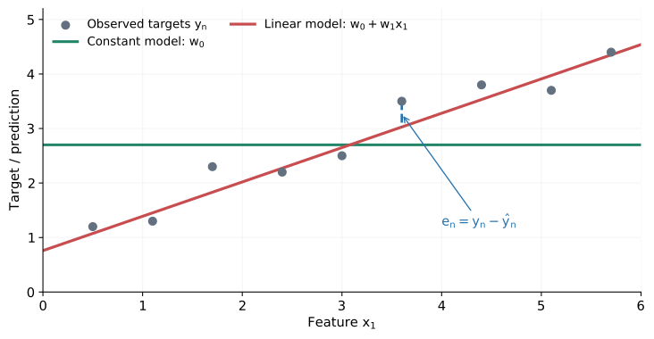
Constant and sloped models for the same observations, with one residual illustrated.
- Each target \(y_n\) may differ from its predicted value \(\hat y_n\).
- Residual: the signed vertical discrepancy.
The residual
\[\boxed{e_n=y_n-\hat y_n=y_n-f_{\mathbf w}(\mathbf x_n)}\]
- \(e_n>0\): underprediction.
- \(e_n<0\): overprediction.
- Signed residuals can cancel when added.
- Need to convert residuals into a penalty.
Individual loss versus dataset loss
Loss of one observation
\[\ell(e_n)\]
Average over \(N\) observations
\[\boxed{L(\mathbf w)=\frac1N\sum_{n=1}^{N}\ell(e_n)}\]
- Individual loss \(\ell\): penalty for one prediction error.
- Objective \(L(\mathbf w)\): one number for the whole dataset.
What does learning minimize?
\[\boxed{L(\mathbf w)=\frac1N\sum_{n=1}^{N}\ell\!\left(y_n-f_{\mathbf w}(\mathbf x_n)\right)}\]
\[\mathbf w^*\in\operatorname*{arg\,min}_{\mathbf w}L(\mathbf w)\]
- Choose what counts as an error.
- Choose how strongly to penalize it.
- Then find suitable parameters.
2 WHAT MAKES A GOOD LOSS?
- Nonnegative; preferably \(\ell(0)=0\).
- Often symmetric: \(\ell(e)=\ell(-e)\).
- Should respond to large mistakes.
- Should not always let a few outliers dominate.
- Should be practical to minimize.
Do positive and negative errors cost the same?
\[\ell(+a)\stackrel{?}{=}\ell(-a)\]
- Symmetry is reasonable for many ordinary regressions.
- Not universal: underpredicting and overpredicting may have different consequences.
- Important to align the loss with the application.
Compare error penalties
![]()
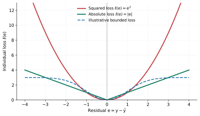
Squared error, absolute error, and a bounded illustrative penalty.
- Squared loss: rapidly increasing penalty.
- Absolute loss: linear increase in magnitude.
- Bounded penalty: illustrative way to reduce extreme-error influence.
Statistical versus computational trade-off
Statistical side
- Does the loss fit the typical data?
- Can a few atypical measurements distort the model?
Computational side
- Can we efficiently minimize the resulting objective?
- Are properties such as convexity useful?
3 MEAN SQUARED ERROR (MSE)
Individual squared loss
\[\ell_{\mathrm{SE}}(e_n)=e_n^2\]
Mean over the dataset
\[\boxed{\mathrm{MSE}(\mathbf w)=\frac1N\sum_{n=1}^{N}(y_n-\hat y_n)^2=\frac1N\sum_{n=1}^{N}e_n^2}\]
- Positive and negative residuals penalized equally.
- Double error magnitude → four times the loss.
MSE: a one-parameter exercise
Constant model
\[\hat y_n=w_0\]
Observed targets
\[\mathbf y=(1,2,3,4)^\top\]
- \(N=4\): input features do not affect this model.
- Try candidate parameters \(w_0=1,2,\ldots,7\).
MSE: work through one candidate
At \(w_0=1\):
\[\begin{aligned}e_1&=1-1=0 &e_2&=2-1=1\\e_3&=3-1=2 &e_4&=4-1=3\end{aligned}\]
\[\sum_{n=1}^{4}e_n^2=0^2+1^2+2^2+3^2=14\]
\[\mathrm{MSE}(1)=14/4=3.5\]
MSE: try the remaining parameters
| Squared-error sum |
14 |
6 |
6 |
14 |
30 |
54 |
86 |
- Best among these integer candidates: \(w_0=2\) or \(3\).
- Continuous optimum: \(w_0=2.5\) (the mean target).
- Sum and mean have the same minimizers for fixed \(N\).
Add one very different observation
\[\mathbf y=(1,2,3,4,\color{red}{20})^\top\]
- Fifth point: unusually large target.
- At \(w_0=2\), new point contributes:
\[\color{red}{(20-2)^2=324}\]
- Does it change the best-fitting parameter?
MSE with the outlier
| Four-point sum |
14 |
6 |
6 |
14 |
30 |
54 |
86 |
| Outlier contribution |
361 |
324 |
289 |
256 |
225 |
196 |
169 |
| Five-point sum |
375 |
330 |
295 |
270 |
255 |
250 |
255 |
- New optimum: \(w_0=6\).
- Original continuous optimum: \(2.5\).
- One extreme observation can substantially change the fit.
MSE: why the fitted value changes
![]()
MSE objectives before and after adding the outlier 20.
- Constant-model MSE minimizer = mean target.
- \((1+2+3+4)/4=2.5\).
- \((1+2+3+4+20)/5=6\).
4 OUTLIERS AND ROBUSTNESS
An outlier is unusually far from the main body of observations.
- May be rare but real.
- May result from faulty measurements or data handling.
- No universal numeric threshold for every dataset.
- Loss choice affects how much outliers influence the fit.
Historical measurement example
![]()
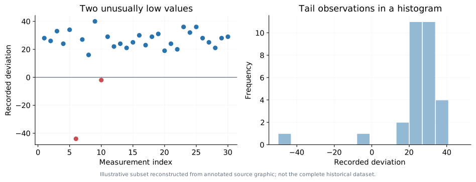
Illustrative reconstruction of unusual recorded values associated with Newcomb’s measurements.
- Historical speed-of-light data contained unusual values \(-44\) and \(-2\) in recorded deviation units.
- These are not negative physical speeds.
- Figure is illustrative, not the complete historical dataset.
Robustness: the question
- Should one or two points determine most of the model fit?
- How should we handle unexplained large residuals?
- We still want to correct meaningful large errors.
- Next: absolute error as a different penalty.
5 MEAN ABSOLUTE ERROR (MAE)
Individual absolute loss
\[\ell_{\mathrm{AE}}(e_n)=|e_n|\]
Mean over the dataset
\[\boxed{\mathrm{MAE}(\mathbf w)=\frac1N\sum_{n=1}^{N}|y_n-\hat y_n|=\frac1N\sum_{n=1}^{N}|e_n|}\]
- Symmetric, nonnegative.
- Double error magnitude → twice the loss.
MAE: the same four observations
\[\mathbf y=(1,2,3,4)^\top,\qquad \hat y_n=w_0\]
| Absolute-error sum |
6 |
4 |
4 |
6 |
10 |
14 |
18 |
- Best integer candidates: 2 and 3.
- Over real values: every \(w_0\in[2,3]\) is optimal.
MAE: now add the target 20
| Four-point sum |
6 |
4 |
4 |
6 |
10 |
14 |
18 |
| Extra contribution |
19 |
18 |
17 |
16 |
15 |
14 |
13 |
| Five-point sum |
25 |
22 |
21 |
22 |
25 |
28 |
31 |
- Optimal constant prediction: \(w_0=3\).
- Only a small shift from original optimum interval.
MAE: why the fit is more stable here
![]()
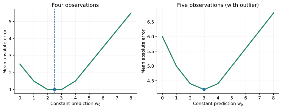
MAE objectives before and after adding the outlier 20.
- Constant-model MAE minimizer = median.
- Median less sensitive to an extreme value’s magnitude.
- Not automatically the best loss for every problem.
Compare MSE and MAE
| Individual penalty |
\(e^2\) |
\(|e|\) |
| Large-error growth |
Quadratic |
Linear |
| Constant-model fit |
Mean |
Median |
| Outlier influence |
Stronger |
More controlled |
| At \(e=0\) |
Smooth |
Corner |
| Convex in \(e\)? |
Yes |
Yes |
Think: which loss is preferable?
- Most measurements reliable; large errors important → MSE may fit the goal.
- Extreme residuals should have less influence → MAE may help.
- Smoothness makes MSE convenient for gradients.
- MAE remains optimizable, even with its corner at zero.
Losses encode practical consequences
- Is an overprediction as costly as an underprediction?
- Financial decisions: two types of wrong decisions may carry different costs.
- Engineering decisions: safety consequences may be asymmetric.
- Choose the objective to reflect what matters in the application.
Training and validation loss
- Training loss: computed on data used for model fitting.
- Validation loss: computed on held-out observations.
- Same metric can reveal whether performance carries over to new cases.
- Loss functions matter beyond regression: classification and other tasks.
6 CONVEXITY
Statistical desirability is only half the problem: can we minimize the objective?
- We optimize \(L(\mathbf w)\) over model parameters.
- Convexity helps avoid inferior local minima.
- Must examine the full model + loss combination.
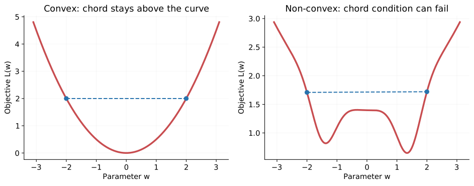
What is a convex function?
Geometric idea
- Draw any two points on the function.
- The chord joining them lies on or above the curve.
Geometric check: convex or not?
![]()
Chord criterion for convex versus non-convex functions.
- A convex curve stays below its chords.
- A non-convex curve can rise above a chord.
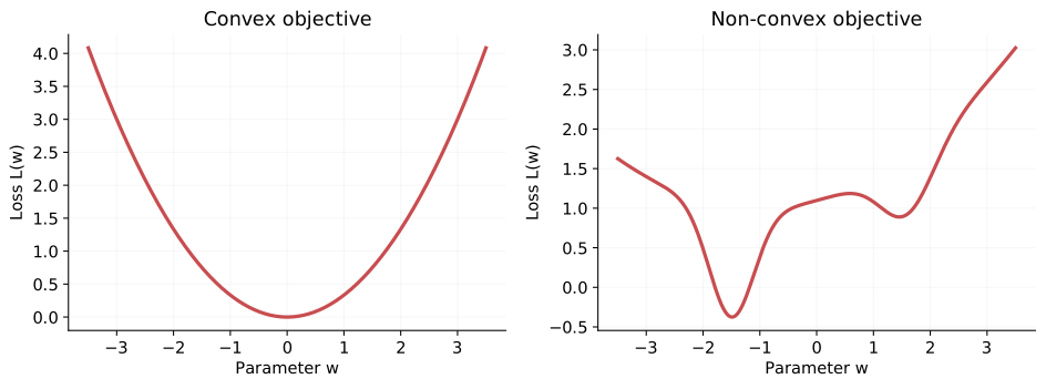
Why is convexity useful?
- Convex objective: every local minimum is global.
- Non-convex objective: different local minima may have different loss values.
- Strictly convex + attained minimum: unique minimizer.
![]()
Convex and non-convex objectives.
Convexity of loss versus objective
Individual loss:
\[\ell(e_n)\]
Full fitting objective:
\[L(\mathbf w)=\frac1N\sum_{n=1}^{N}\ell\!\left(y_n-f_{\mathbf w}(\mathbf x_n)\right)\]
- Optimization variable: \(\mathbf w\).
- Convexity of \(\ell(e)\) alone is not enough for an arbitrary model.
Squared loss with a linear model
Let \(f_{\mathbf w}(\mathbf x_n)=\mathbf x_n^\top\mathbf w\).
\[L_{\mathrm{MSE}}(\mathbf w)=\frac1N\sum_{n=1}^{N}\left(y_n-\mathbf x_n^\top\mathbf w\right)^2\]
- Residual is affine in \(\mathbf w\).
- Squared affine residual: convex in \(\mathbf w\).
- Average of convex terms: convex objective.
But is the solution always unique?
- Convex \(\neq\) strictly convex.
- Dependent features or too few independent observations → possibly multiple optima.
- Recall Chapter 2: overparameterization.
- Convex optimization may be tractable without a unique parameter vector.
Exercise: MAE with a linear model
Can you establish convexity in \(\mathbf w\)?
\[\ell_n(\mathbf w)=\left|y_n-\mathbf x_n^\top\mathbf w\right|\]
- Choose parameter vectors \(\mathbf u\), \(\mathbf v\).
- Consider their convex combination.
- Use the triangle inequality.
Exercise: key inequality
\[\begin{aligned}
&\left|y_n-\mathbf x_n^\top(\lambda\mathbf u+(1-\lambda)\mathbf v)\right|\\
&\quad\leq \lambda|y_n-\mathbf x_n^\top\mathbf u|+(1-\lambda)|y_n-\mathbf x_n^\top\mathbf v|
\end{aligned}\]
- MAE + linear model: convex in the parameters.
- The corner at zero does not destroy convexity.
- Both MSE and MAE are convex here.
7 THE PRACTICAL TRADE-OFF
MSE
- Smooth, straightforward derivatives.
- Can be strongly affected by outliers.
MAE
- More controlled influence of extreme residuals.
- Corner at zero; still convex and optimizable.
Other losses
- Can be designed for even greater robustness.
- Some lead to non-convex objectives.
Optional reading: beyond MSE and MAE
- Huber loss: squared behavior near zero, linear for larger errors.
- Tukey bisquare: bounded robust penalty; can be non-convex.
- Additional design choices, including thresholds.
- Not part of the core derivations in this chapter.
Chapter summary
- Residual \(e_n=y_n-\hat y_n\) → individual loss \(\ell(e_n)\).
- Dataset objective \(L(\mathbf w)=N^{-1}\sum_n\ell(e_n)\).
- MSE: quadratic penalty; constant fit selects mean.
- MAE: linear penalty; constant fit selects median.
- Outliers affect these fits differently.
- Convexity simplifies optimization but does not ensure a unique solution.
Check your understanding
- Residual versus individual versus dataset loss?
- Why square errors or take absolute values?
- MSE versus MAE under the outlier \(20\)?
- What does convexity guarantee about local minima?
- Is the MAE objective convex for linear regression?
- Why might the practical cost of errors be asymmetric?
Coming next
Optimization
- We now know what to minimize.
- How do we systematically update model parameters?
- When can we efficiently find a good or global minimum?
Acknowledgements and AI Disclosure
Acknowledgements
- Developed with reference to CS-433 Machine Learning, École Polytechnique Fédérale de Lausanne (EPFL).
- Adapted and extended for the present course, including civil engineering applications.
- Independent teaching materials; no EPFL endorsement is implied.
- Original EPFL course
Use of Generative AI
- AI-assisted drafting, editing, examples, figures, and interactive visualizations.
- The instructor is responsible for the final content and technical accuracy.
- External materials are acknowledged separately.